   fza  fzt vc       lc       Ra
1 0.50 0.10 40 emulsion 1.915556
2 1.25 0.10 40 emulsion 3.515556
3 0.50 0.20 40 emulsion 1.065556
4 1.25 0.20 40 emulsion 1.965556
5 0.50 0.15 20 emulsion 1.765556
6 1.25 0.15 20 emulsion 3.265556Ra modeling with SVM radial - Helical milling of Inconel 718 with round carbide inserts
Loading libraries, defining experimental design, and getting measurement results.
The same as done previously.
Tuning best model again with a wider grid
The best model was the SVM radial. Tuning with a wider grid is performed to improve model performance. A grid of 10 values of both cost and \(\sigma\) is considered.
normalized_rec <-
  recipe(Ra ~ ., data = plan_train) %>%
  step_normalize(fza,fzt,vc) %>%
  step_dummy(all_nominal_predictors())

svm_r_spec <-
  svm_rbf(cost = tune(), rbf_sigma = tune()) %>%
  set_engine("kernlab") %>%
  set_mode("regression")

svm_wflow <-
  workflow() %>%
    add_model(svm_r_spec) %>%
  add_recipe(normalized_rec)

p <- parameters(cost(), rbf_sigma())

param_grid <- grid_regular(p, levels = 10)

tune_res <- tune_grid(
  svm_wflow,
  resamples = plan_folds,
  grid = param_grid
)autoplot(tune_res) + theme_bw()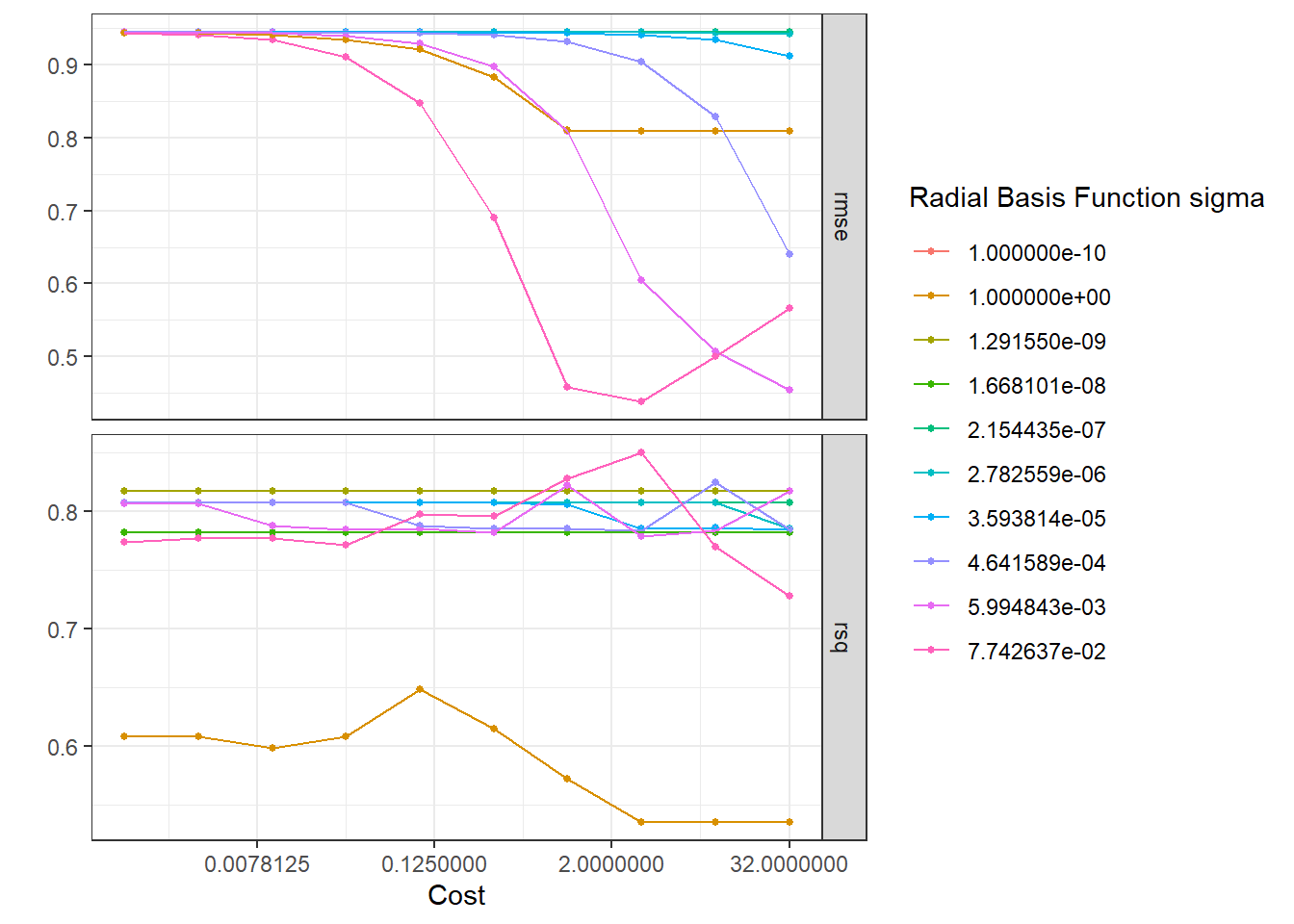
collect_metrics(tune_res) %>%
  arrange(mean)
# A tibble: 200 × 8
cost rbf_sigma .metric .estimator mean n std_err .config
<dbl> <dbl> <chr> <chr> <dbl> <int> <dbl> <chr>
1 3.17 0.0774 rmse standard 0.438 20 0.0673 Preprocessor1_Model088
2 32 0.00599 rmse standard 0.454 20 0.0676 Preprocessor1_Model080
3 1 0.0774 rmse standard 0.459 20 0.0749 Preprocessor1_Model087
4 10.1 0.0774 rmse standard 0.501 20 0.0638 Preprocessor1_Model089
5 10.1 0.00599 rmse standard 0.507 20 0.0697 Preprocessor1_Model079
6 10.1 1 rsq standard 0.535 20 0.0680 Preprocessor1_Model099
7 32 1 rsq standard 0.535 20 0.0680 Preprocessor1_Model100
8 3.17 1 rsq standard 0.535 20 0.0679 Preprocessor1_Model098
9 32 0.0774 rmse standard 0.566 20 0.0697 Preprocessor1_Model090
10 1 1 rsq standard 0.572 20 0.0786 Preprocessor1_Model097
# ℹ 190 more rowsbest_rmse <-
tune_res %>%
select_best(metric = "rmse")
best_rmse# A tibble: 1 × 3
cost rbf_sigma .config
<dbl> <dbl> <chr>
1 3.17 0.0774 Preprocessor1_Model088best_rsq <-
tune_res %>%
select_best(metric = "rsq")
best_rsq# A tibble: 1 × 3
cost rbf_sigma .config
<dbl> <dbl> <chr>
1 3.17 0.0774 Preprocessor1_Model088The best model considering both rmse and rsq is with cost = 3.174802 and \(\sigma = 0.07742637\).
svm_r_final <- finalize_workflow(svm_wflow, best_rmse)

svm_r_final_fit <- fit(svm_r_final, data = plan_train)
Final model is then defined with these parameters’ levels.
augment(svm_r_final_fit, new_data = plan_test) %>%
  rsq(truth = Ra, estimate = .pred)
# A tibble: 1 × 3
.metric .estimator .estimate
<chr> <chr> <dbl>
1 rsq standard 0.894augment(svm_r_final_fit, new_data = plan_test) %>%
rmse(truth = Ra, estimate = .pred)# A tibble: 1 × 3
.metric .estimator .estimate
<chr> <chr> <dbl>
1 rmse standard 0.300Evaluating the model in the whole training set
The model is evaluated in the whole training data set.
svm_r_res <- predict(svm_r_final_fit, new_data = plan_train %>% select(-Ra))
svm_r_res <- bind_cols(svm_r_res, plan_train %>% select(Ra))
head(svm_r_res)
# A tibble: 6 × 2
.pred Ra
<dbl> <dbl>
1 1.87 1.92
2 3.61 3.52
3 0.967 1.07
4 2.06 1.97
5 3.17 3.27
6 1.26 1.17ggplot(svm_r_res, aes(x = Ra, y = .pred)) +
# Create a diagonal line:
geom_abline(lty = 2) +
geom_point(alpha = 0.5) +
coord_obs_pred() + theme_bw()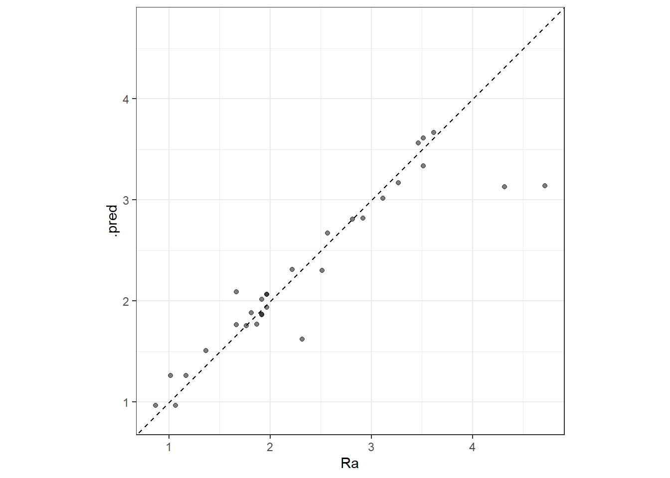
Model interpretation
Effects plots to interpret the model according to process aspects.
##########
x1_grid <- seq(min(plan_train$fza), max(plan_train$fza), length = 50)
ypred_fza_em <- predict(svm_r_final_fit, new_data = data.frame(fza = x1_grid,
                                                               fzt = 0.15,
                                                               vc = 40,
                                                               lc = "emulsion"))
data_p1_em <- data.frame(fza = x1_grid,
                         Ra = ypred_fza_em$.pred,
                         fzt = 0.15,
                         vc = 40,
                         lc = "emulsion")

ypred_fza_mql <- predict(svm_r_final_fit, new_data = data.frame(fza = x1_grid,
                                                                fzt = 0.15,
                                                                vc = 40,
                                                                lc = "mql"))
data_p1_mql <- data.frame(fza = x1_grid,
                      Ra = ypred_fza_mql$.pred,
                      fzt = 0.15,
                      vc = 40,
                      lc = "mql")

data_p1 <- rbind(data_p1_em, data_p1_mql)

p1 <- ggplot(data = data_p1, mapping = aes(x = fza, y = Ra, group = lc)) +
  geom_line(aes(colour = lc, linetype = lc), linewidth = 1.2) +
  ylim(.8,2.9) +
  scale_color_manual(values = c("red", "blue")) +
  theme_bw()

##########
x2_grid <- seq(min(plan_train$fzt), max(plan_train$fzt), length = 50)
ypred_fzt_em <- predict(svm_r_final_fit, new_data = data.frame(fza = 0.875,
                                                               fzt = x2_grid,
                                                               vc = 40,
                                                               lc = "emulsion"))
data_p2_em <- data.frame(fza = 0.875,
                         Ra = ypred_fzt_em$.pred,
                         fzt = x2_grid,
                         vc = 40,
                         lc = "emulsion")

ypred_fzt_mql <- predict(svm_r_final_fit, new_data = data.frame(fza = 0.875,
                                                                fzt = x2_grid,
                                                                vc = 40,
                                                                lc = "mql"))
data_p2_mql <- data.frame(fza = 0.875,
                          Ra = ypred_fzt_mql$.pred,
                          fzt = x2_grid,
                          vc = 40,
                          lc = "mql")

data_p2 <- rbind(data_p2_em, data_p2_mql)

p2 <- ggplot(data = data_p2, mapping = aes(x = fzt, y = Ra, group = lc)) +
  geom_line(aes(colour = lc, linetype = lc), linewidth = 1.2) +
  ylim(.8,2.9) +
  scale_color_manual(values = c("red", "blue")) +
  theme_bw()

##########
x3_grid <- seq(min(plan_train$vc), max(plan_train$vc), length = 50)
ypred_vc_em <- predict(svm_r_final_fit, new_data = data.frame(fza = 0.875,
                                                               fzt = 0.15,
                                                               vc = x3_grid,
                                                               lc = "emulsion"))
data_p3_em <- data.frame(fza = 0.875,
                         Ra = ypred_fzt_em$.pred,
                         fzt = 0.15,
                         vc = x3_grid,
                         lc = "emulsion")

ypred_vc_mql <- predict(svm_r_final_fit, new_data = data.frame(fza = 0.875,
                                                                fzt = 0.15,
                                                                vc = x3_grid,
                                                                lc = "mql"))
data_p3_mql <- data.frame(fza = 0.875,
                          Ra = ypred_vc_mql$.pred,
                          fzt = 0.15,
                          vc = x3_grid,
                          lc = "mql")

data_p3 <- rbind(data_p3_em, data_p3_mql)

p3 <- ggplot(data = data_p3, mapping = aes(x = vc, y = Ra, group = lc)) +
  geom_line(aes(colour = lc, linetype = lc), linewidth = 1.2) +
  ylim(.8,2.9) +
  scale_color_manual(values = c("red", "blue")) +
  theme_bw()

ggarrange(p1, p2 , p3, common.legend = TRUE, nrow = 1)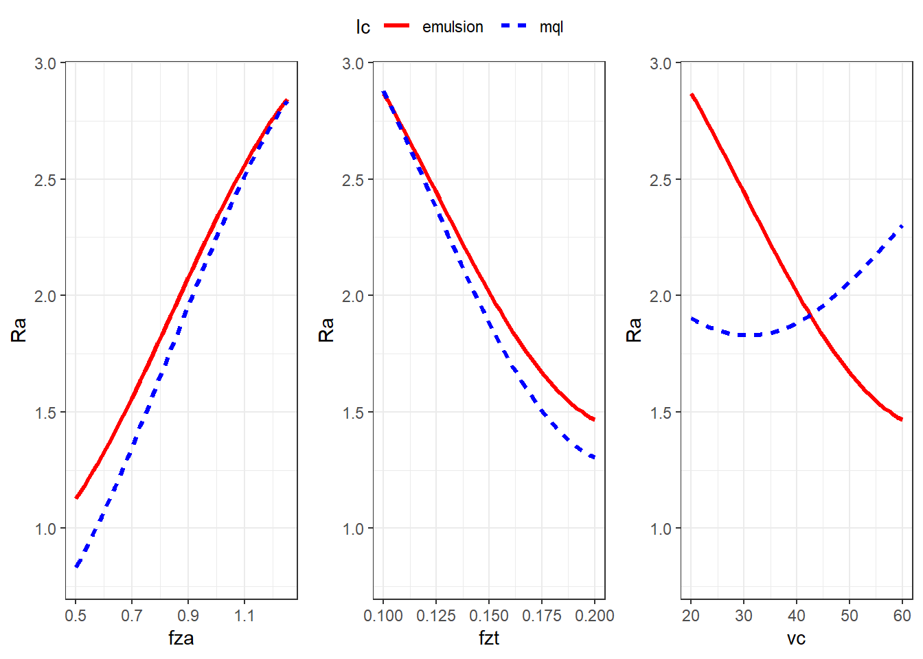
ypred_fza_em_a <- predict(svm_r_final_fit, new_data = data.frame(fza = x1_grid,
                                                                 fzt = 0.1,
                                                                 vc = 40,
                                                                 lc = "emulsion"))
data_p1_em_a <- data.frame(fza = x1_grid,
                           Ra = ypred_fza_em_a$.pred,
                           fzt = 0.1,
                           vc = 40,
                           lc = "emulsion")

ypred_fza_mql_a <- predict(svm_r_final_fit, new_data = data.frame(fza = x1_grid,
                                                                  fzt = 0.1,
                                                                  vc = 40,
                                                                  lc = "mql"))
data_p1_mql_a <- data.frame(fza = x1_grid,
                            Ra = ypred_fza_mql_a$.pred,
                            fzt = 0.1,
                            vc = 40,
                            lc = "mql")

ypred_fza_em_b <- predict(svm_r_final_fit, new_data = data.frame(fza = x1_grid,
                                                                 fzt = 0.2,
                                                                 vc = 40,
                                                                 lc = "emulsion"))
data_p1_em_b <- data.frame(fza = x1_grid,
                           Ra = ypred_fza_em_b$.pred,
                           fzt = 0.2,
                           vc = 40,
                           lc = "emulsion")

ypred_fza_mql_b <- predict(svm_r_final_fit, new_data = data.frame(fza = x1_grid,
                                                                  fzt = 0.2,
                                                                  vc = 40,
                                                                  lc = "mql"))
data_p1_mql_b <- data.frame(fza = x1_grid,
                            Ra = ypred_fza_mql_b$.pred,
                            fzt = 0.2,
                            vc = 40,
                            lc = "mql")

data_p1_fza_fzt <- rbind(data_p1, data_p1_em_a, data_p1_mql_a,
                         data_p1_em_b, data_p1_mql_b)

pp12 <- ggplot(data_p1_fza_fzt, aes(y = Ra, x = fza, group = fzt)) +
  geom_line(aes(color = fzt), linewidth = 1.2) +
  # scale_fill_binned(type = "viridis") +
  scale_color_gradient(low="blue", high="red") +
  facet_grid(cols = vars(lc), scales = "free") +
  ylim(.6,3.8) +
  theme_bw()
ypred_fza_em_c <- predict(svm_r_final_fit, new_data = data.frame(fza = x1_grid,
fzt = 0.15,
vc = 20,
lc = "emulsion"))
data_p1_em_c <- data.frame(fza = x1_grid,
Ra = ypred_fza_em_c$.pred,
fzt = 0.15,
vc = 20,
lc = "emulsion")
ypred_fza_mql_c <- predict(svm_r_final_fit, new_data = data.frame(fza = x1_grid,
fzt = 0.15,
vc = 20,
lc = "mql"))
data_p1_mql_c <- data.frame(fza = x1_grid,
Ra = ypred_fza_mql_c$.pred,
fzt = 0.15,
vc = 20,
lc = "mql")
ypred_fza_em_d <- predict(svm_r_final_fit, new_data = data.frame(fza = x1_grid,
fzt = 0.15,
vc = 60,
lc = "emulsion"))
data_p1_em_d <- data.frame(fza = x1_grid,
Ra = ypred_fza_em_d$.pred,
fzt = 0.15,
vc = 60,
lc = "emulsion")
ypred_fza_mql_d <- predict(svm_r_final_fit, new_data = data.frame(fza = x1_grid,
fzt = 0.15,
vc = 60,
lc = "mql"))
data_p1_mql_d <- data.frame(fza = x1_grid,
Ra = ypred_fza_mql_d$.pred,
fzt = 0.15,
vc = 60,
lc = "mql")
data_p1_fza_vc <- rbind(data_p1, data_p1_em_c, data_p1_mql_c,
data_p1_em_d, data_p1_mql_d)
pp13 <- ggplot(data_p1_fza_vc, aes(y = Ra, x = fza, group = vc)) +
geom_line(aes(color = vc), linewidth = 1.2) +
scale_color_gradient(low="blue", high="red") +
facet_grid(cols = vars(lc), scales = "free") +
ylim(.6,3.8) +
theme_bw()ypred_fzt_em_c <- predict(svm_r_final_fit, new_data = data.frame(fza = 0.875,
fzt = x2_grid,
vc = 20,
lc = "emulsion"))
data_p2_em_c <- data.frame(fza = 0.875,
fzt = x2_grid,
Ra = ypred_fzt_em_c$.pred,
vc = 20,
lc = "emulsion")
ypred_fzt_mql_c <- predict(svm_r_final_fit, new_data = data.frame(fza = 0.875,
fzt = x2_grid,
vc = 20,
lc = "mql"))
data_p2_mql_c <- data.frame(fza = 0.875,
fzt = x2_grid,
Ra = ypred_fzt_mql_c$.pred,
vc = 20,
lc = "mql")
ypred_fzt_em_d <- predict(svm_r_final_fit, new_data = data.frame(fza = 0.875,
fzt = x2_grid,
vc = 60,
lc = "emulsion"))
data_p2_em_d <- data.frame(fza = 0.875,
fzt = x2_grid,
Ra = ypred_fzt_em_d$.pred,
vc = 60,
lc = "emulsion")
ypred_fzt_mql_d <- predict(svm_r_final_fit, new_data = data.frame(fza = 0.875,
fzt = x2_grid,
vc = 60,
lc = "mql"))
data_p2_mql_d <- data.frame(fza = 0.875,
fzt = x2_grid,
Ra = ypred_fzt_mql_d$.pred,
vc = 60,
lc = "mql")
data_p2_fzt_vc <- rbind(data_p2, data_p2_em_c, data_p2_mql_c,
data_p2_em_d, data_p2_mql_d)
pp23 <- ggplot(data_p2_fzt_vc, aes(y = Ra, x = fzt, group = vc)) +
geom_line(aes(color = vc), linewidth = 1.2) +
scale_color_gradient(low="blue", high="red") +
facet_grid(cols = vars(lc), scales = "free") +
ylim(.6,3.8) +
theme_bw()ggarrange(pp12,pp13,pp23, nrow = 3)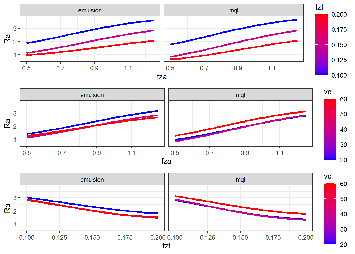
Contour plots.
#######################
grid_12_em <- expand.grid(fza = x1_grid,
                          fzt = x2_grid,
                          vc = 40, lc = "emulsion")
y_hat_12_em <- predict(svm_r_final_fit, new_data = grid_12_em)
grid_12_em$Ra <- y_hat_12_em$.pred


grid_12_mql <- expand.grid(fza = x1_grid,
                           fzt = x2_grid,
                           vc = 40, lc = "mql")
y_hat_12_mql <- predict(svm_r_final_fit, new_data = grid_12_mql)
grid_12_mql$Ra <- y_hat_12_mql$.pred


grid_12 <- rbind(grid_12_em, grid_12_mql)


cp12 <- ggplot(data = grid_12,
                  mapping = aes(x = fza, y = fzt, z = Ra)) +
  geom_tile(aes(fill=Ra)) +
   facet_grid(cols = vars(lc), scales = "free") +
  scale_fill_distiller(palette = "RdBu",
                       direction = -1) +
  geom_contour(color = "black") +
  theme_bw()

#######################
grid_13_em <- expand.grid(fza = x1_grid,
                          fzt = 0.15,
                          vc = x3_grid, lc = "emulsion")
y_hat_13_em <- predict(svm_r_final_fit, new_data = grid_13_em)
grid_13_em$Ra <- y_hat_13_em$.pred


grid_13_mql <- expand.grid(fza = x1_grid,
                          fzt = 0.15,
                          vc = x3_grid, lc = "mql")
y_hat_13_mql <- predict(svm_r_final_fit, new_data = grid_13_mql)
grid_13_mql$Ra <- y_hat_13_mql$.pred


grid_13 <- rbind(grid_13_em, grid_13_mql)


cp13 <- ggplot(data = grid_13,
                  mapping = aes(x = fza, y = vc, z = Ra)) +
  geom_tile(aes(fill=Ra)) +
   facet_grid(cols = vars(lc), scales = "free") +
  scale_fill_distiller(palette = "RdBu",
                       direction = -1) +
  geom_contour(color = "black") +
  theme_bw()


#######################
grid_23_em <- expand.grid(fza = 0.875,
                          fzt = x2_grid,
                          vc = x3_grid, lc = "emulsion")
y_hat_23_em <- predict(svm_r_final_fit, new_data = grid_23_em)
grid_23_em$Ra <- y_hat_23_em$.pred


grid_23_mql <- expand.grid(fza = 0.875,
                           fzt = x2_grid,
                           vc = x3_grid, lc = "mql")
y_hat_23_mql <- predict(svm_r_final_fit, new_data = grid_23_mql)
grid_23_mql$Ra <- y_hat_23_mql$.pred


grid_23 <- rbind(grid_23_em, grid_23_mql)


cp23 <- ggplot(data = grid_23,
                  mapping = aes(x = fzt, y = vc, z = Ra)) +
  geom_tile(aes(fill=Ra)) +
   facet_grid(cols = vars(lc), scales = "free") +
  scale_fill_distiller(palette = "RdBu",
                       direction = -1) +
  geom_contour(color = "black") +
  theme_bw()

ggarrange(cp12,cp13,cp23, nrow = 3)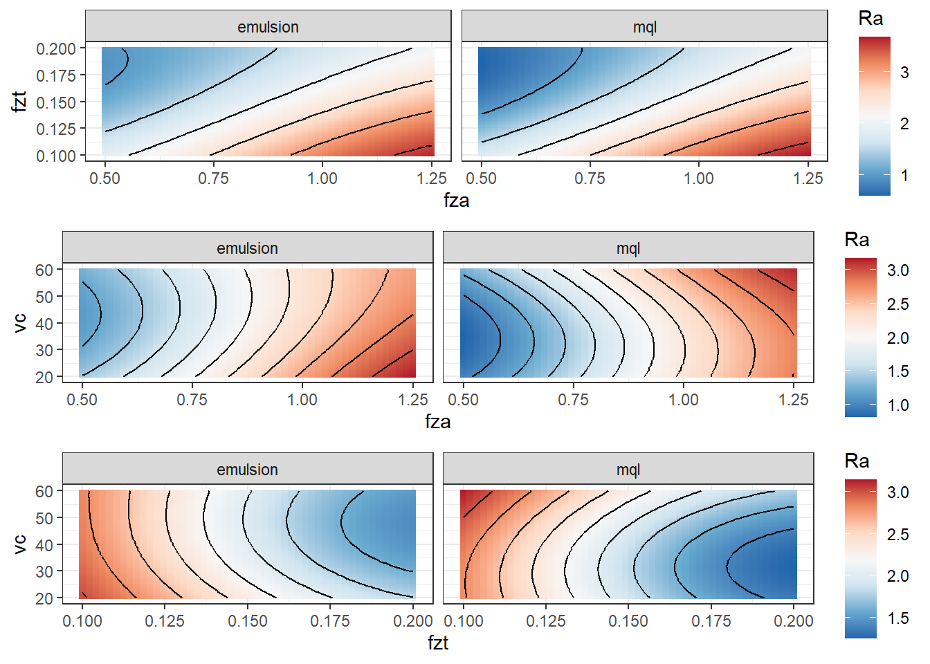
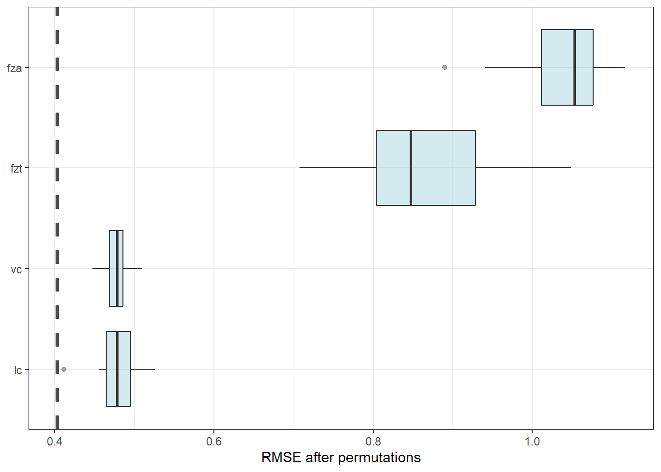
Variance importance plots.
vip_features <- c("fza", "fzt", "vc", "lc")

vip_train <-
  plan_train %>%
  select(all_of(vip_features))

explainer_svm_r<-
  explain_tidymodels(
    svm_r_final_fit,
    data = plan_train %>% select(-Ra),
    y = plan_train$Ra,
    verbose = FALSE
  )

set.seed(1803)
vip_svm <- model_parts(explainer_svm_r, loss_function = loss_root_mean_square)
ggplot_imp <- function(...) {
obj <- list(...)
metric_name <- attr(obj[[1]], "loss_name")
metric_lab <- paste(metric_name,
"after permutations\n(higher indicates more important)")
full_vip <- bind_rows(obj) %>%
filter(variable != "_baseline_")
perm_vals <- full_vip %>%
filter(variable == "_full_model_") %>%
group_by(label) %>%
summarise(dropout_loss = mean(dropout_loss))
p <- full_vip %>%
filter(variable != "_full_model_") %>%
mutate(variable = fct_reorder(variable, dropout_loss)) %>%
ggplot(aes(dropout_loss, variable))
if(length(obj) > 1) {
p <- p +
facet_wrap(vars(label)) +
geom_vline(data = perm_vals, aes(xintercept = dropout_loss, color = label),
linewidth = 1.4, lty = 2, alpha = 0.7) +
geom_boxplot(aes(color = label, fill = label), alpha = 0.2)
} else {
p <- p +
geom_vline(data = perm_vals, aes(xintercept = dropout_loss),
linewidth = 1.4, lty = 2, alpha = 0.7) +
geom_boxplot(fill = "#91CBD765", alpha = 0.4)
}
p +
theme(legend.position = "none") +
labs(x = metric_lab,
y = NULL, fill = NULL, color = NULL)
}ggplot_imp(vip_svm) + labs(x = "RMSE after permutations") + theme_bw()